HMM and PHMM in R
Qian Feng
2018-02-11
Last updated: 2018-02-11
Code version: 4d59175
The ‘aphid’ R package for analysis with profile hidden Markov models is published by Shaun Wilkinson on 2017-06-23. Let’s practice this package to drive HMM and PHMM model and use related algorithms.
library("aphid")
states <- c("Begin", "Fair", "Loaded")
residues <- paste(1:6)
### Define transition probability matrix A
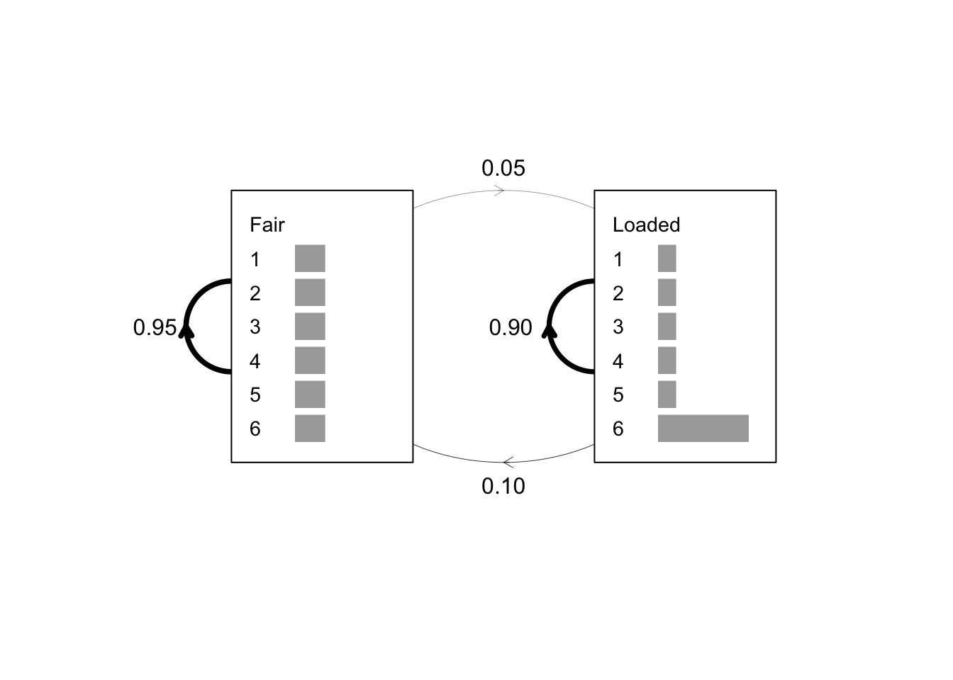
A <- matrix(c(0, 0, 0, 0.99, 0.95, 0.1, 0.01, 0.05, 0.9), nrow = 3)
dimnames(A) <- list(from = states, to = states)
### Define emission probability matrix E
E <- matrix(c(rep(1/6, 6), rep(1/10, 5), 1/2), nrow = 2, byrow = TRUE)
dimnames(E) <- list(states = states[-1], residues = residues)
### Create the HMM object
x <- structure(list(A = A, E = E), class = "HMM")
### Plot the model
plot(x, textexp = 1.5)
### Optionally add the transition probabilities as text
text(x = 0.02, y = 0.5, labels = "0.95")
text(x = 0.51, y = 0.5, labels = "0.90")
text(x = 0.5, y = 0.9, labels = "0.05")
text(x = 0.5, y = 0.1, labels = "0.10")
#### viterbi algorithm
data(casino)
### The actual path is stored in the names attribute of the sequence
actual <- c("F", "L")[match(names(casino), c("Fair", "Loaded"))]
### Find the predicted path
vit1 <- Viterbi(x, casino)
predicted <- c("F", "L")[vit1$path + 1]
### Note the path element of the output Viterbi object is an integer vector
### the addition of 1 to the path converts from C/C++ to R's indexing style
actual[1:50]###list examples fromm first roll to 50th roll
[1] "F" "F" "F" "F" "F" "F" "F" "F" "F" "F" "F" "F" "F" "F" "F" "F" "F"
[18] "F" "F" "F" "F" "F" "F" "F" "F" "F" "F" "F" "F" "F" "F" "F" "F" "F"
[35] "F" "F" "F" "F" "F" "F" "F" "F" "F" "F" "F" "L" "L" "L" "L" "L"predicted[1:50] [1] "F" "F" "F" "F" "F" "F" "F" "F" "F" "F" "F" "F" "F" "F" "F" "F" "F"
[18] "F" "F" "F" "F" "F" "F" "F" "F" "F" "F" "F" "F" "F" "F" "F" "F" "F"
[35] "F" "F" "F" "F" "F" "F" "F" "F" "F" "F" "F" "F" "F" "F" "L" "L"#### forward and posterior probability
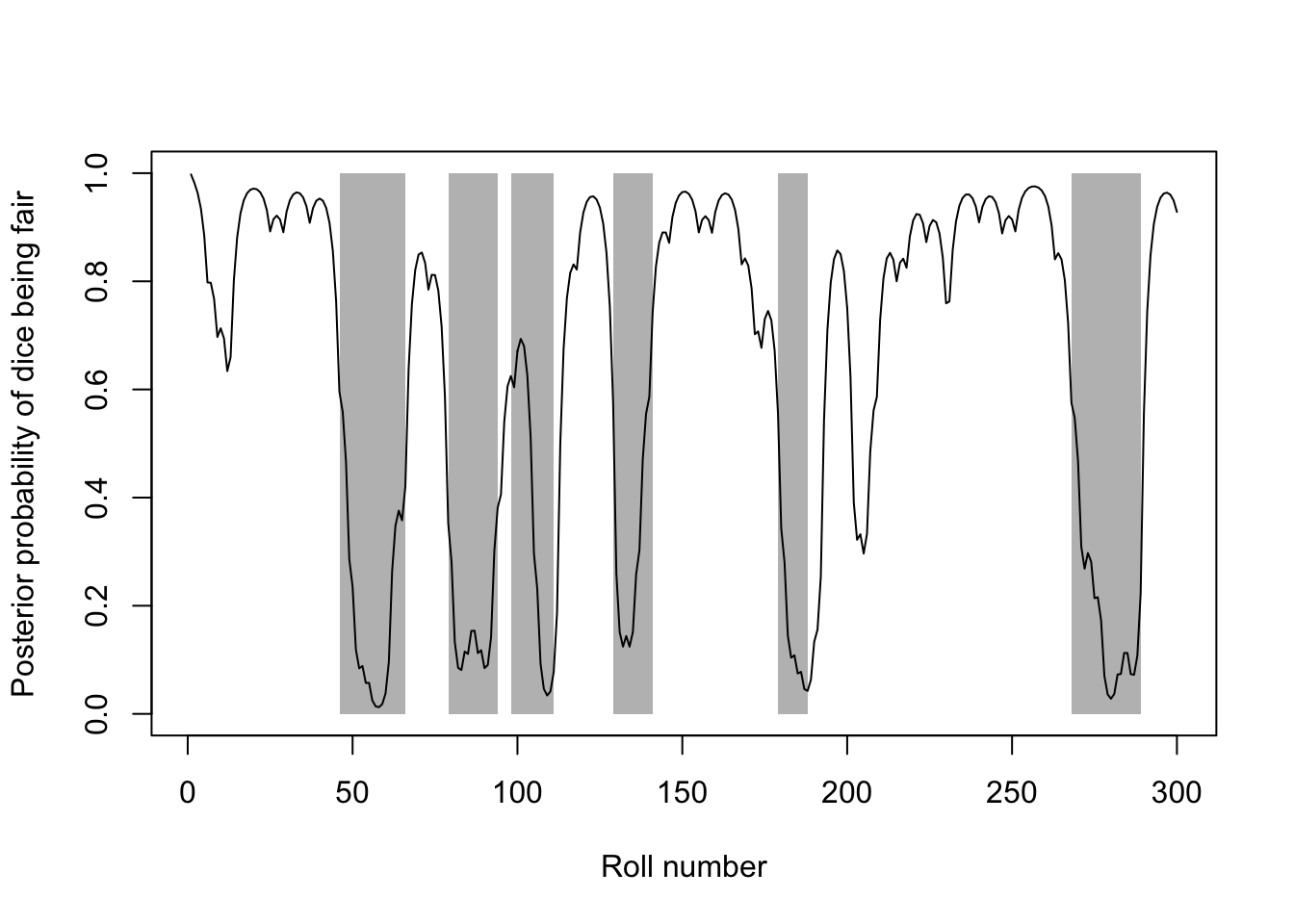
### The line shows the posterior probability that the dice was fair at each roll,
### while the grey rectangles show the actual periods for which the loaded dice
### was being used.
casino.post <- posterior(x, casino)
plot(1:300, seq(0, 1, length.out = 300), type = "n", xlab = "Roll number",
ylab = "Posterior probability of dice being fair")
starts <- which(c("L", actual) == "F" & c(actual, "F") == "L")
ends <- which(c("F", actual) == "L" & c(actual, "L") == "F") - 1
for(i in 1:6) rect(starts[i], 0, ends[i], 1, col = "grey", border = NA)
lines(1:300, casino.post[1, ])
Drive HMM model
#### drive HMM model given a sequence with its known state path
### (stored as the ‘names’ attribute of the sequence)
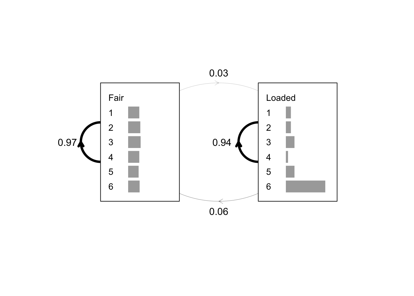
y <- deriveHMM(list(casino), logspace = FALSE)
plot(y, textexp = 1.5)
### Optionally add the transition probabilities as text
text(x = 0.02, y = 0.5, labels = round(y$A["Fair", "Fair"], 2))
text(x = 0.51, y = 0.5, labels = round(y$A["Loaded", "Loaded"], 2))
text(x = 0.5, y = 0.9, labels = round(y$A["Fair", "Loaded"], 2))
text(x = 0.5, y = 0.1, labels = round(y$A["Loaded", "Fair"], 2))
Drive Profile HMM model
#### drive profile HMM model
###“path” element taking values 0 (“delete”), 1 (“match”) or 2 (“insert”)
data(globins)
globins
[,1] [,2] [,3] [,4] [,5] [,6] [,7] [,8] [,9] [,10]
HBA_HUMAN "V" "G" "A" "-" "-" "H" "A" "G" "E" "Y"
HBB_HUMAN "V" "-" "-" "-" "-" "N" "V" "D" "E" "V"
MYG_PHYCA "V" "E" "A" "-" "-" "D" "V" "A" "G" "H"
GLB3_CHITP "V" "K" "G" "-" "-" "-" "-" "-" "-" "D"
GLB5_PETMA "V" "Y" "S" "-" "-" "T" "Y" "E" "T" "S"
LGB2_LUPLU "F" "N" "A" "-" "-" "N" "I" "P" "K" "H"
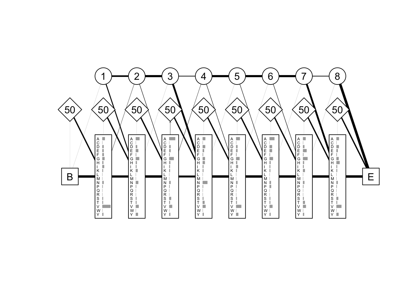
GLB1_GLYDI "I" "A" "G" "A" "D" "N" "G" "A" "G" "V" globins.PHMM <- derivePHMM(globins, residues = "AMINO", seqweights = NULL)
plot(globins.PHMM)
path <- Viterbi(globins.PHMM, globins["GLB1_GLYDI", ])$path
c("D", "M", "I")[path + 1]
[1] "M" "M" "M" "I" "I" "M" "M" "M" "M" "M"Sequence Simulation
#### Sequence Simulation
###generate()is used to generate sequences
###train() is for optimizing model parameters using either the Baum Welch or Viterbi training algorithm
sim <- list(length = 10)
set.seed(9999)
for(i in 1:10) sim[[i]] <- generate(globins.PHMM, size = 20)
sim <- lapply(sim, function(s) s[names(s) != "D"])
globins2.PHMM <- train(globins.PHMM, sim, method = "BaumWelch",
                       deltaLL = 0.01, seqweights = NULL)
Iteration 1 log likelihood = -213.8818
Iteration 2 log likelihood = -188.625
Iteration 3 log likelihood = -187.6561
Iteration 4 log likelihood = -187.1078
Iteration 5 log likelihood = -186.8872
Iteration 6 log likelihood = -186.8454
Iteration 7 log likelihood = -186.8401
Convergence threshold reached after 7 EM iterationsSequence Alignment
#### Sequence Alignment
##deconstruct the original globin alignment and re-align the sequences using the original PHMM.
globins <- unalign(globins)
align(globins, model = globins.PHMM, seqweights = NULL, residues = "AMINO")
1 2 3 I I 4 5 6 7 8
HBA_HUMAN "V" "G" "A" "-" "-" "H" "A" "G" "E" "Y"
HBB_HUMAN "V" "-" "-" "-" "-" "N" "V" "D" "E" "V"
MYG_PHYCA "V" "E" "A" "-" "-" "D" "V" "A" "G" "H"
GLB3_CHITP "V" "K" "G" "-" "-" "-" "-" "-" "-" "D"
GLB5_PETMA "V" "Y" "S" "-" "-" "T" "Y" "E" "T" "S"
LGB2_LUPLU "F" "N" "A" "-" "-" "N" "I" "P" "K" "H"
GLB1_GLYDI "I" "A" "G" "A" "D" "N" "G" "A" "G" "V"Session information
sessionInfo()R version 3.4.2 (2017-09-28)
Platform: x86_64-apple-darwin15.6.0 (64-bit)
Running under: macOS Sierra 10.12.1
Matrix products: default
BLAS: /Library/Frameworks/R.framework/Versions/3.4/Resources/lib/libRblas.0.dylib
LAPACK: /Library/Frameworks/R.framework/Versions/3.4/Resources/lib/libRlapack.dylib
locale:
[1] zh_CN.UTF-8/zh_CN.UTF-8/zh_CN.UTF-8/C/zh_CN.UTF-8/zh_CN.UTF-8
attached base packages:
[1] stats graphics grDevices utils datasets methods base
other attached packages:
[1] aphid_1.0.1
loaded via a namespace (and not attached):
[1] compiler_3.4.2 backports_1.1.2 magrittr_1.5 rprojroot_1.3-2
[5] tools_3.4.2 htmltools_0.3.6 yaml_2.1.16 Rcpp_0.12.14
[9] stringi_1.1.6 rmarkdown_1.8 knitr_1.18 git2r_0.21.0
[13] stringr_1.2.0 digest_0.6.14 openssl_0.9.9 evaluate_0.10.1This R Markdown site was created with workflowr